The Sum Over 1 Problem

I recently came across this fun probability problem which I’ve dubbed the ‘Sum Over 1’ problem.

It goes like this:

On average, how many random draws from the interval [0, 1] are necessary to ensure that their sum exceeds 1?

To answer this question we’ll use some probability theory (probability rules, distribution functions, expected value) and a dash of calculus (integration).

Let’s Begin!

Let $U_i$ follow a Uniform distribution over the interval $[0, 1]$, where $i = 1, 2, \ldots$ denotes the $i^{\text{th}}$ draw.

Let $N$ denote the number of draws such that $\sum_{i=1}^{N} U_i > 1$ and $\sum_{i=1}^{N-1} U_i \leq 1$. Thus, $N$ is a discrete random variable taking values $n=2,3,\ldots$ ($n=1$ is impossible because no single draw from $[0, 1]$ can exceed 1).

We seek the long-run average, or expected value, of $N$ denoted $E(N)$. A good first step for a numerical problem like this is to utilize computer simulations to point us in the right direction.

Simulations with R

Let’s generate, say, 20 random draws from $[0,1]$, $(u_1, \ldots, u_{20})$.

draws <- runif(20)  # vector of u_1, ..., u_20

Consider the partial sums of these draws $(u_1, u_1 + u_2, \sum_{i=1}^3 u_i, \ldots, \sum_{i=1}^{20} u_i)$.

If we index this partial sum vector from 1 up to 20, then $n$ here is simply the index of the first component of this vector whose value exceeds 1.

The find_n function accomplishes this for any vector of random draws u:

find_n <- function(u) {
  which(cumsum(u) > 1)[1]  # which partial sum first exceeds 1?
}

n <- find_n(draws)
draws[1:n]

## [1] 0.2858056 0.1689087 0.6259122

In this instance, it took 3 random draws from $[0, 1]$ to sum over 1. We can sample from the probability distribution of $N$ by repeating this process many more times. The sample_from_N function takes m samples from the distribution of $N$:

sample_from_N <- function(m) {
  # m-by-20 matrix of random [0,1] draws
  draws <- matrix(runif(m * 20), ncol = 20)
  # for each row of 20 draws, find n
  n.many <- apply(draws, 1, find_n)
  # estimate P(N = n), n = 2, 3, ..., 10
  # (truncated b/c probs are miniscule for n > 10)
  estimated.probs <- table(factor(n.many, levels = 2:10)) / m  
  return(estimated.probs)
}

m <- 1000
approx.N <- sample_from_N(m)  # approximate prob. dist'n of N
approx.N

## 
##     2     3     4     5     6     7     8     9    10 
## 0.514 0.330 0.121 0.026 0.005 0.004 0.000 0.000 0.000

So, we estimate $P(N = 2)$ by $\hat{P}(N = 2) = 0.514$, $P(N = 3)$ by $\hat{P}(N = 3) = 0.33$, and so forth.

These are just point estimates for $P(N = n)$, but we can estimate their standard errors as well by running sample_from_N many more times. The approximate probability distribution of $N$ is depicted below.

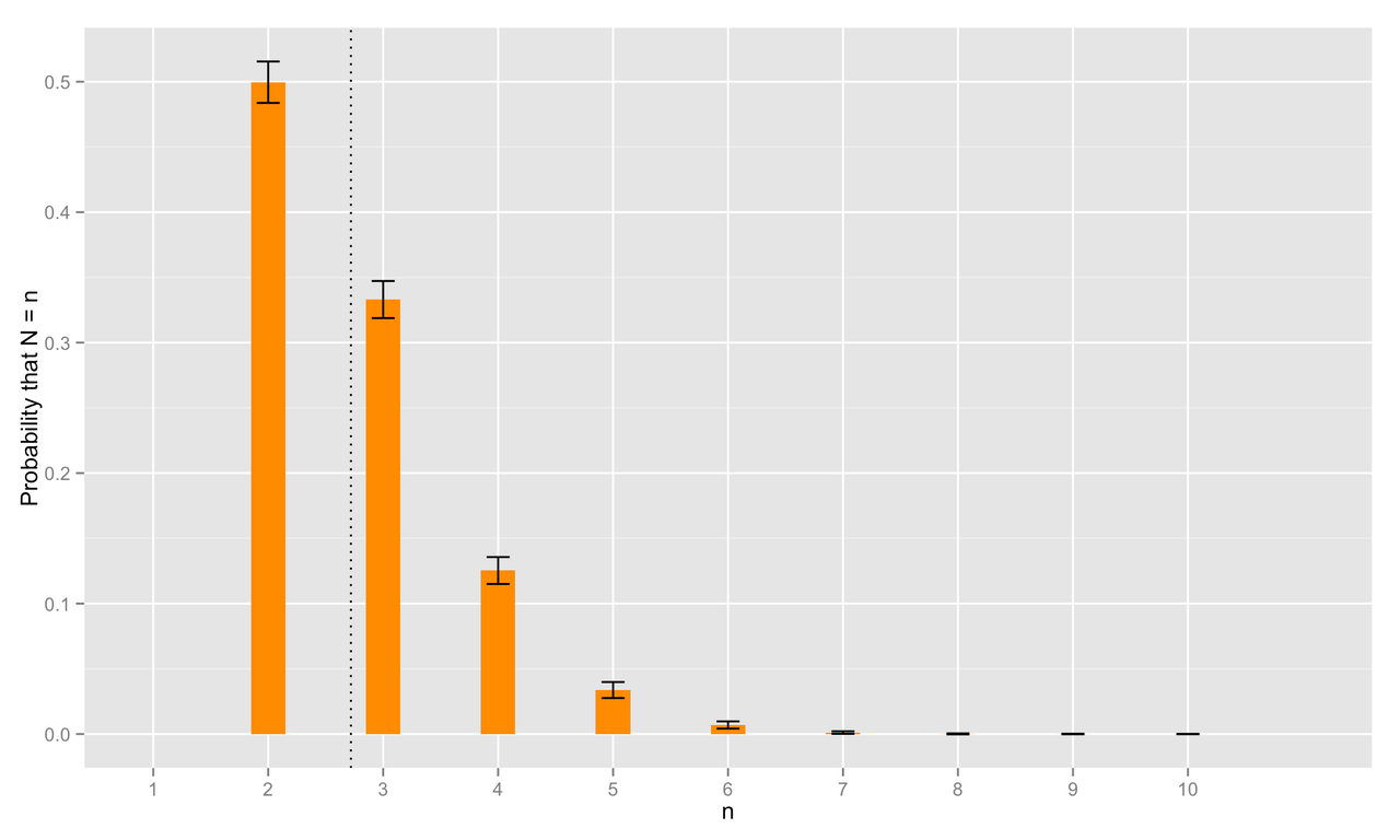
The dotted line here marks the estimated expected value of $N$, $\hat{E}(N) = \sum_{n=2}^{\infty} n\hat{P}(N=n) \approx 2.71962$. This value is tantalizingly close to the mathematical constant $e\approx 2.7183$ known as Euler’s number¹.

Could the answer to our probability puzzle truly be $e$?

Proof

Let’s start small by finding the probability that $N=2$. The probability that it takes exactly 2 random draws from $[0, 1]$ for their sum to exceed 1 is simply the complement of the probability that the sum of our 2 draws fall short of exceeding 1. That is,

$$\begin{equation} P(N = 2) = P(U_1 + U_2 > 1) = 1 - P(U_1 + U_2 \leq 1). \end{equation}$$

We can interpret the probability that $U_1 + U_2 \leq 1$ geometrically. Since $U_1$ and $U_2$ are Uniform random variables on $[0, 1]$, the point $(U_1, U_2)$ can arise anywhere in the unit square with equal probability. Thus, $P(U_1 + U_2 \leq 1)$ corresponds exactly to the proportion of the unit square shaded in the following image.

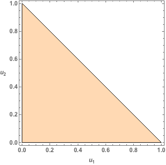
This shaded region is referred to as a 2-dimensional unit simplex² with area

So $P(N=2) = 1 - 1/2 = 1/2$, which agrees nicely with our simulation estimate $\hat{P}(N = 2) = 0.514$.

Now for the probability that $N=3$, it is tempting to proceed by finding the exact probability

but dealing with both inequality constraints simultaneously is annoying. It is helpful to recognize that $P(N = 3) = P(N \leq 3) - P(N = 2)$ where

Similar to the previous case, the probability that the sum of three random draws from [0,1], $U_1, U_2,$ and $U_3$, does not exceed 1 is given by the proportion of the unit cube shaded in the following image.

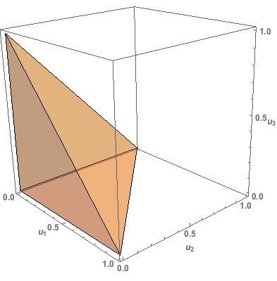
This shaded region is a 3-dimensional unit simplex with volume

So $P(N=3) = P(N\leq 3) - P(N=2) = (1 - 1/6) - 1/2 = 1/3$ which again agrees with our simulation estimate of $\hat{P}(N = 3) = 0.33$.

Foregoing a formal proof, we can generalize our results on the unit simplex: the $n$-dimensional unit simplex has “volume” given by $1 / n!$. For our purposes, $P(N \leq n) = 1 - 1/n!$. Thus, for any $n\geq 2$,

We’ve got everything we need to find the expected value of $N$.

Recall the exponential series is given by $e^{x} = \sum_{n=0}^{\infty} \frac{x^{n}}{n!}$.

Thus, $E(N)$ is equivalently $e$.

Yes that’s right: we expect, on average, $e$ random draws from the interval $[0, 1]$ to ensure their sum exceeds 1!