Neal Grantham
Fill the region between two lines in ggplot2
Update (2022-05-09): This blog post presents the “Unbraided Ribbon Problem” in ggplot2 and my first attempt at a solution to it. It received a lot of positive feedback on Twitter — the “Unbraided Ribbon Problem” is more common than I thought — and a handful of readers asked if I would consider making this work into an R package. In doing so I discovered that the
ribbonize()function at the end of this post does not work in all cases, so I got to work on a second attempt at a solution. I think I’ve finally solved it! My new package is called ggbraid and you can read more about it at nsgrantham.github.io/ggbraid. Happy braiding!
Last week I searched #ggplot on Twitter looking for a challenge and I found the following tweet:
“This shouldn’t be hard,” I thought. Wrong!
Hugh eventually solved the problem with spatial R packages wk and sf, and shared his code in this GitHub gist.
In this post I present an alternate solution using geom_ribbon() and a custom function I’ve written called ribbonize().
The Case of the Missing Regions
I’ll use the same fake data that Hugh used in his tweet, but I’ve renamed the variables.
library(tidyverse)  # 1.3.1

df <- tibble(
  x = c(1:6, 1:6),
  y = c(1, 5, 6, 4, 1, 1, 1, 4, 5, 4, 2, 2),
  f = c(rep("a", 6), rep("b", 6))
)

df
## # A tibble: 12 × 3
##        x     y f
##    <int> <dbl> <chr>
##  1     1     1 a
##  2     2     5 a
##  3     3     6 a
##  4     4     4 a
##  5     5     1 a
##  6     6     1 a
##  7     1     1 b
##  8     2     4 b
##  9     3     5 b
## 10     4     4 b
## 11     5     2 b
## 12     6     2 b
Let’s plot df with ggplot(). Map x to x, y to y and f to linetype. Apply the line geometry with geom_line().
ggplot(df) +
  geom_line(aes(x, y, linetype = f)) +
  guides(linetype = "none") +
  labs(x = NULL, y = NULL)
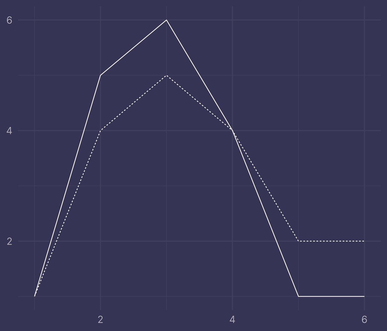
To fill the regions between these two lines with geom_ribbon(), we’ll need to define a data frame with variables that we can map to the following aesthetics: x, ymax, ymin, and fill.
In this case, it’s easiest to pivot df wider so that the levels in f become two different columns with values from y. Then we use pairwise max and min, pmax and pmin, to find ymax and ymin respectively. We define the fill variable to be a >= b so that it takes values TRUE and FALSE.
bounds <- df %>%
  pivot_wider(names_from = f, values_from = y) %>%
  mutate(
    ymax = pmax(a, b),
    ymin = pmin(a, b),
    fill = a >= b
  )

bounds
## # A tibble: 6 × 6
##       x     a     b  ymax  ymin fill
##   <int> <dbl> <dbl> <dbl> <dbl> <lgl>
## 1     1     1     1     1     1 TRUE
## 2     2     5     4     5     4 TRUE
## 3     3     6     5     6     5 TRUE
## 4     4     4     4     4     4 TRUE
## 5     5     1     2     2     1 FALSE
## 6     6     1     2     2     1 FALSE
Take the previous plot and add a new layer to it by applying geom_ribbon() to bounds and mapping x to x, ymin to ymin, ymax to ymax, and fill to fill. Also, include some transparency in the colors with alpha = 0.4.
ggplot(df) +
  geom_line(aes(x, y, linetype = f)) +
  geom_ribbon(data = bounds, aes(x, ymin = ymin, ymax = ymax, fill = fill), alpha = 0.4) +
  guides(linetype = "none", fill = "none") +
  labs(x = NULL, y = NULL)
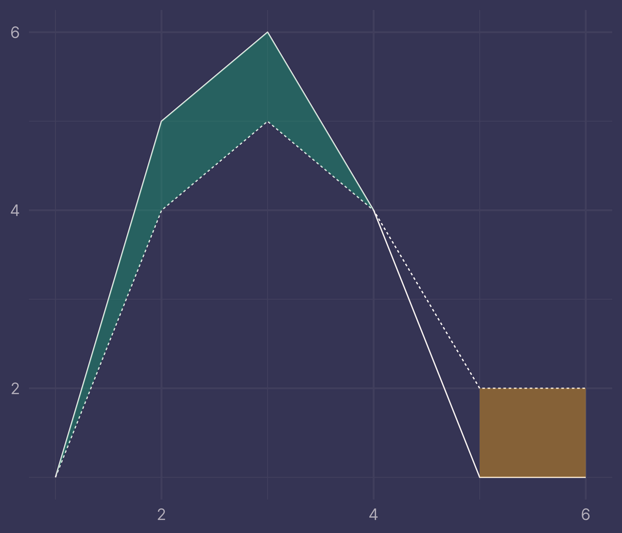
Ugh. That’s not right. What did we do wrong?
I tracked down a GitHub issue from 2016 that describes the problem we’re facing. There is some discussion on what is causing this. “I don’t think this is a ggplot2 bug, I think this is expected behavior,” comments @jonocarroll. @hadley weighs in, acknowledging the behavior and suggesting that “this is better fixed outside of ggplot2.”
As far as I can tell, this problem hasn’t been fixed inside or outside of ggplot2 in the 5 years since this GitHub issue was opened.
It’s Not a Bug, It’s a Feature
The first question to ask is: why is this happening?
Let’s take another look at bounds.
bounds
## # A tibble: 6 × 6
##       x     a     b  ymax  ymin fill
##   <int> <dbl> <dbl> <dbl> <dbl> <lgl>
## 1     1     1     1     1     1 TRUE
## 2     2     5     4     5     4 TRUE
## 3     3     6     5     6     5 TRUE
## 4     4     4     4     4     4 TRUE
## 5     5     1     2     2     1 FALSE
## 6     6     1     2     2     1 FALSE
When x is 1, 2, 3, or 4, fill is TRUE and geom_ribbon() fills the region between the intersections at x = 1 and x = 4.
When x is 5 or 6, fill is FALSE and geom_ribbon() fills the region between these two values (with a different color than when fill is TRUE).
But what about the region between 4 and 5? There’s nothing in bounds that would tell geom_ribbon() to fill this region — as far as it knows, fill = TRUE between x = 1 and x = 4 and fill = FALSE between x = 5 and x = 6.
We must append a new row to bounds so geom_ribbon() knows that fill = FALSE begins at x = 4, not x = 5.
bounds2 <- bind_rows(
  bounds,
  tibble(x = 4, a = 4, b = 4, ymax = 4, ymin = 4, fill = FALSE)
) %>%
  arrange(x)

bounds2
## # A tibble: 7 × 6
##       x     a     b  ymax  ymin fill
##   <dbl> <dbl> <dbl> <dbl> <dbl> <lgl>
## 1     1     1     1     1     1 TRUE
## 2     2     5     4     5     4 TRUE
## 3     3     6     5     6     5 TRUE
## 4     4     4     4     4     4 TRUE
## 5     4     4     4     4     4 FALSE
## 6     5     1     2     2     1 FALSE
## 7     6     1     2     2     1 FALSE
ggplot(df) +
  geom_line(aes(x, y, linetype = f)) +
  geom_ribbon(data = bounds2, aes(x, ymin = ymin, ymax = ymax, fill = fill), alpha = 0.4) +
  guides(linetype = "none", fill = "none") +
  labs(x = NULL, y = NULL)
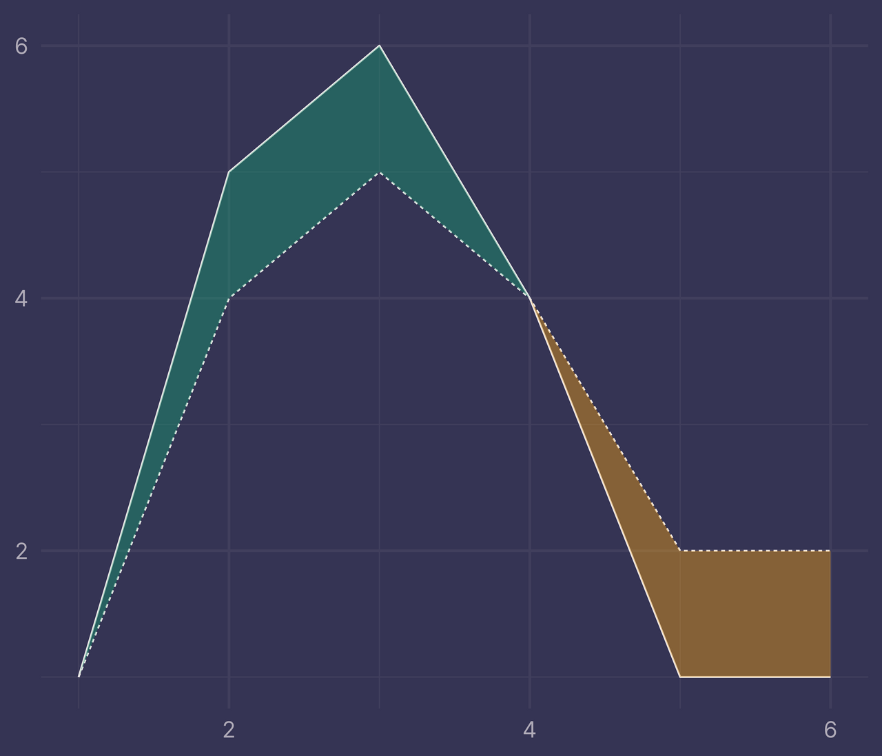
Success!
So the problem is not caused by a bug in ggplot2.
The real problem is that we were not passing the right data to geom_ribbon() so it was unable to fill the regions correctly.
Intervals and Intersections
Now the next question to ask is: how do I get the right data?
There are many ways to approach this. Of course, we can stick with the manual approach above, adding new rows to bounds as they’re required. But ideally we’d find a programmatic way to get the right data every time.
To do so, it’s helpful to separate bounds into two different data frames: intervals and intersections.
Filter bounds on ymax > ymin and assign it to intervals.
intervals <- bounds %>%
  filter(ymax > ymin)

intervals
## # A tibble: 4 × 6
##       x     a     b  ymax  ymin fill
##   <int> <dbl> <dbl> <dbl> <dbl> <lgl>
## 1     2     5     4     5     4 TRUE
## 2     3     6     5     6     5 TRUE
## 3     5     1     2     2     1 FALSE
## 4     6     1     2     2     1 FALSE
Leave intervals alone (since it already behaves correctly when passed to geom_ribbon()).
Next, filter bounds on ymax == ymin and assign it to intersections.
intersections <- bounds %>%
  filter(ymax == ymin)

intersections
## # A tibble: 2 × 6
##       x     a     b  ymax  ymin fill
##   <int> <dbl> <dbl> <dbl> <dbl> <lgl>
## 1     1     1     1     1     1 TRUE
## 2     4     4     4     4     4 TRUE
intersections requires some additional work to get right.
We have an intersection at x = 1 where fill = TRUE begins.
We also have an intersection at x = 4 where fill = TRUE ends and fill = FALSE begins. However, only fill = TRUE is captured in intersections so we must transform intersections to include a new row.
To do so, we will use arrange() to sort the rows of bounds by x and define two new variables, lag_fill and lead_fill, which record the previous and next fill values respectively.
intersections <- bounds %>%
  arrange(x) %>%
  mutate(lag_fill = lag(fill), lead_fill = lead(fill)) %>%
  filter(ymax == ymin)

intersections
## # A tibble: 2 × 8
##       x     a     b  ymax  ymin fill  lag_fill lead_fill
##   <int> <dbl> <dbl> <dbl> <dbl> <lgl> <lgl>    <lgl>
## 1     1     1     1     1     1 TRUE  NA       TRUE
## 2     4     4     4     4     4 TRUE  TRUE     FALSE
When x = 1, lag_fill is NA because there is no previous row and lead_fill is TRUE since fill is TRUE at the next row x = 2.
When x = 4, lag_fill is TRUE because the previous row has x = 3 and fill = TRUE and lead_fill is FALSE because the next row has x = 5 and fill = FALSE.
Now, we can pivot longer and replace fill with the values of lag_fill and lead_fill. Further, remove any rows where fill is NA and remove duplicate rows, should they exist, with distinct().
intersections <- bounds %>%
  arrange(x) %>%
  mutate(lag_fill = lag(fill), lead_fill = lead(fill)) %>%
  filter(ymax == ymin) %>%
  select(-fill) %>%
  pivot_longer(lag_fill:lead_fill, names_to = NULL, values_to = "fill") %>%
  filter(!is.na(fill)) %>%
  distinct()

intersections
## # A tibble: 3 × 6
##       x     a     b  ymax  ymin fill
##   <int> <dbl> <dbl> <dbl> <dbl> <lgl>
## 1     1     1     1     1     1 TRUE
## 2     4     4     4     4     4 TRUE
## 3     4     4     4     4     4 FALSE
Bind intervals and intersections to create a new data frame, ribbons, and pass this to geom_ribbon() instead of bounds.
ribbons <- bind_rows(
  intervals,
  intersections
)

ggplot(df) +
  geom_line(aes(x, y, linetype = f)) +
  geom_ribbon(data = ribbons, aes(x, ymin = ymin, ymax = ymax, fill = fill), alpha = 0.4) +
  guides(linetype = "none", fill = "none") +
  labs(x = NULL, y = NULL)

We did it!
Alright, so we’re done?
Not so fast.
Other Intersections
Suppose we add a few new rows to the original data.
df <- tibble(
  x = c(1:8, 1:8),
  y = c(1, 5, 6, 4, 1, 1, 3, 2, 1, 4, 5, 4, 2, 2, 2, 2),
  f = c(rep("a", 8), rep("b", 8))
)

ggplot(df, aes(x, y, linetype = f)) +
  geom_line() +
  guides(linetype = "none") +
  labs(x = NULL, y = NULL)
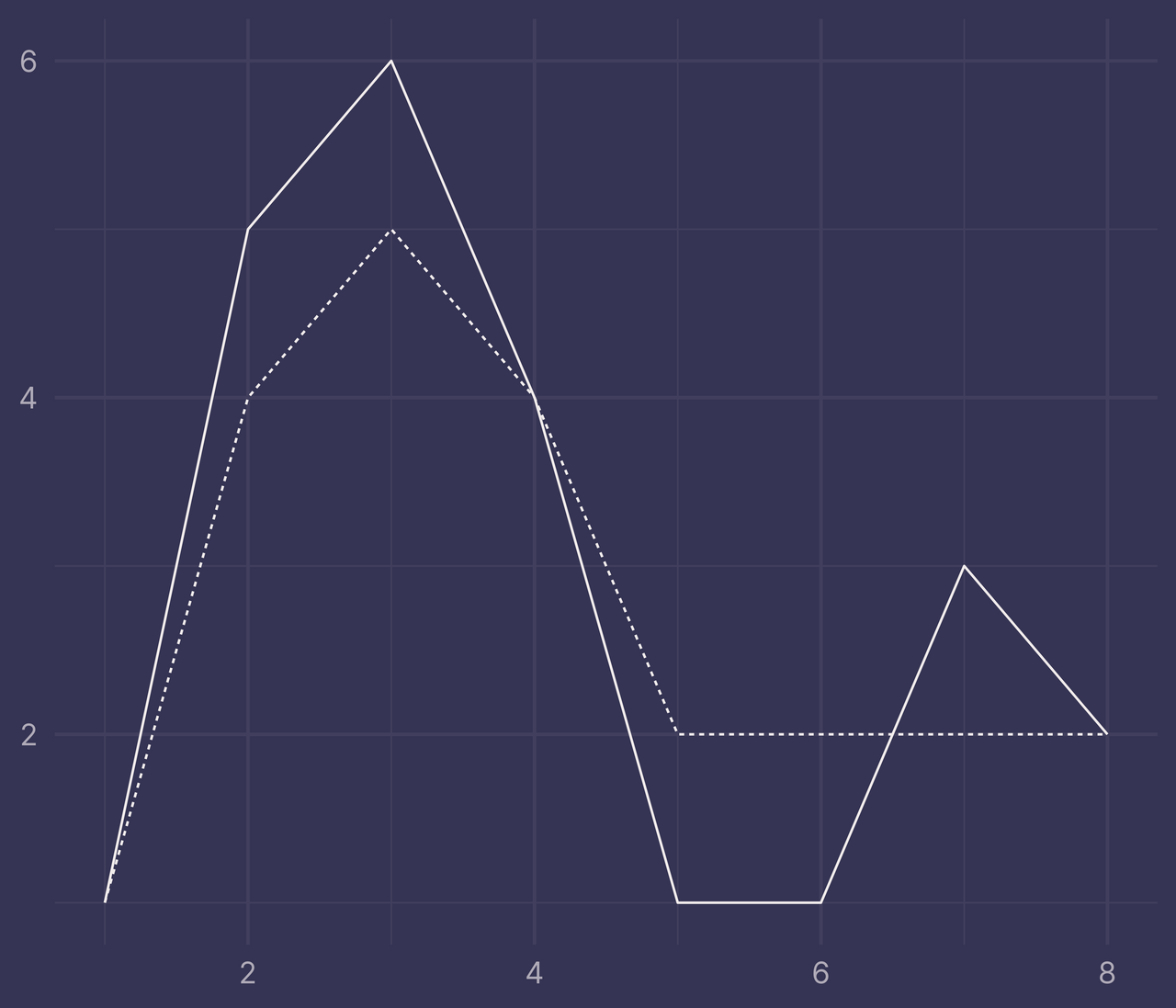
Now repeat the same steps as before with intervals and intersections (but this time we’ll remove the a and b variables when they’re no longer needed).
bounds <- df %>%
  pivot_wider(names_from = f, values_from = y) %>%
  mutate(
    ymax = pmax(a, b),
    ymin = pmin(a, b),
    fill = a > b
  )

intervals <- bounds %>%
  filter(ymax > ymin) %>%
  select(-a, -b)

intersections <- bounds %>%
  mutate(lag_fill = lag(fill), lead_fill = lead(fill)) %>%
  filter(ymax == ymin) %>%
  select(-a, -b, -fill) %>%
  pivot_longer(lag_fill:lead_fill, names_to = NULL, values_to = "fill") %>%
  filter(!is.na(fill)) %>%
  distinct()

ribbons <- bind_rows(
  intervals,
  intersections
) %>%
  arrange(x)

ribbons
## # A tibble: 9 × 4
##       x  ymax  ymin fill
##   <int> <dbl> <dbl> <lgl>
## 1     1     1     1 TRUE
## 2     2     5     4 TRUE
## 3     3     6     5 TRUE
## 4     4     4     4 TRUE
## 5     4     4     4 FALSE
## 6     5     2     1 FALSE
## 7     6     2     1 FALSE
## 8     7     3     2 TRUE
## 9     8     2     2 TRUE
ggplot(df) +
  geom_line(aes(x, y, linetype = f)) +
  geom_ribbon(data = ribbons, aes(x, ymin = ymin, ymax = ymax, fill = fill), alpha = 0.4) +
  guides(linetype = "none", fill = "none") +
  labs(x = NULL, y = NULL)
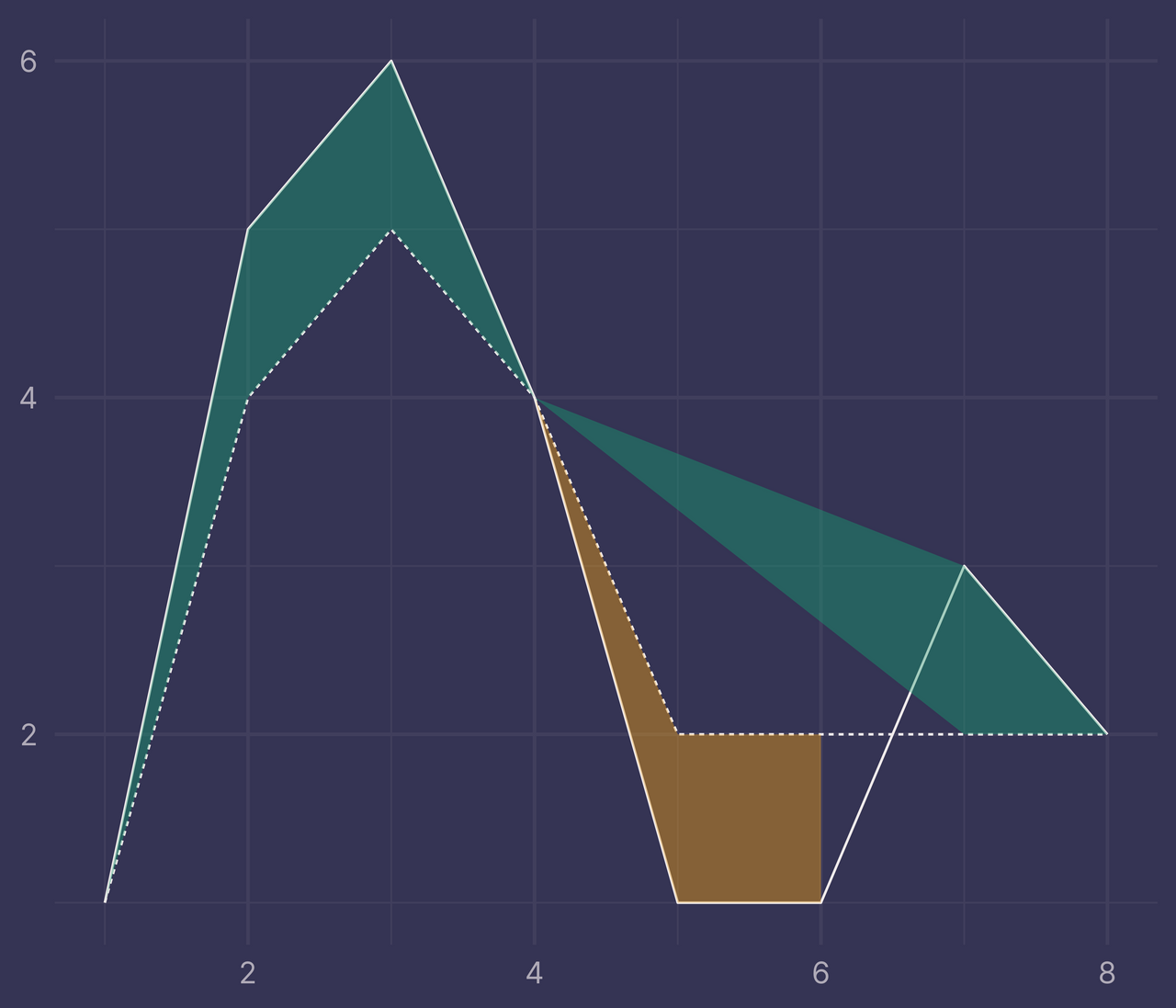
Bleh. It looks kinda cool, but it’s not at all what we want.
So, why is this happening?
There’s a new intersection that occurs at x = 6.5 but we have no such row in ribbons, only x = 6 and x = 7.
To accommodate this new intersection, we’ll need to calculate its position and add it as a new row to ribbons.
Thankfully there’s a formula we can use to find the position of an intersection point given two points on each line.
To make things easier to follow, I’ll use similar variable names as in the formula. The following steps may look a little complicated, but it’s not necessary to follow along completely. Just know that we are applying the formula in a tidy way to find any intersections that occur between two x.
other_intersections <- bounds %>%
  transmute(
    x1 = x,       y1 = a,
    x2 = lead(x), y2 = lead(a),
    x3 = x,       y3 = b,
    x4 = lead(x), y4 = lead(b)
  ) %>%
  filter(((y1 > y3) & (y2 < y4)) | ((y1 < y3) & (y2 > y4))) %>%  # only rows where an intersection occurs between two x
  mutate(
    d = (x1 - x2) * (y3 - y4) - (y1 - y2) * (x3 - x4),  # denominator
    u = x1 * y2 - y1 * x2,
    v = x3 * y4 - y3 * x4,
    x = (u * (x3 - x4) - v * (x1 - x2)) / d,
    y = (u * (y3 - y4) - v * (y1 - y2)) / d
  ) %>%
  select(x, ymax = y, ymin = y)

other_intersections
## # A tibble: 1 × 3
##       x  ymax  ymin
##   <dbl> <dbl> <dbl>
## 1   6.5     2     2
Now points in other_intersections will always mark transitions from fill = TRUE to fill = FALSE or the other way around, so we’ll bind two versions of other_intersections to intervals and intersections, one where fill = TRUE and another where fill = FALSE.
ribbons <- bind_rows(
  intervals,
  intersections,
  mutate(other_intersections, fill = TRUE),
  mutate(other_intersections, fill = FALSE)
) %>%
  arrange(x)

ribbons
## # A tibble: 11 × 4
##        x  ymax  ymin fill
##    <dbl> <dbl> <dbl> <lgl>
##  1   1       1     1 TRUE
##  2   2       5     4 TRUE
##  3   3       6     5 TRUE
##  4   4       4     4 TRUE
##  5   4       4     4 FALSE
##  6   5       2     1 FALSE
##  7   6       2     1 FALSE
##  8   6.5     2     2 TRUE
##  9   6.5     2     2 FALSE
## 10   7       3     2 TRUE
## 11   8       2     2 TRUE
Putting this all together, we plot again and…
ggplot(df) +
  geom_line(aes(x, y, linetype = f)) +
  geom_ribbon(data = ribbons, aes(x, ymin = ymin, ymax = ymax, fill = fill), alpha = 0.4) +
  guides(linetype = "none", fill = "none") +
  labs(x = NULL, y = NULL)
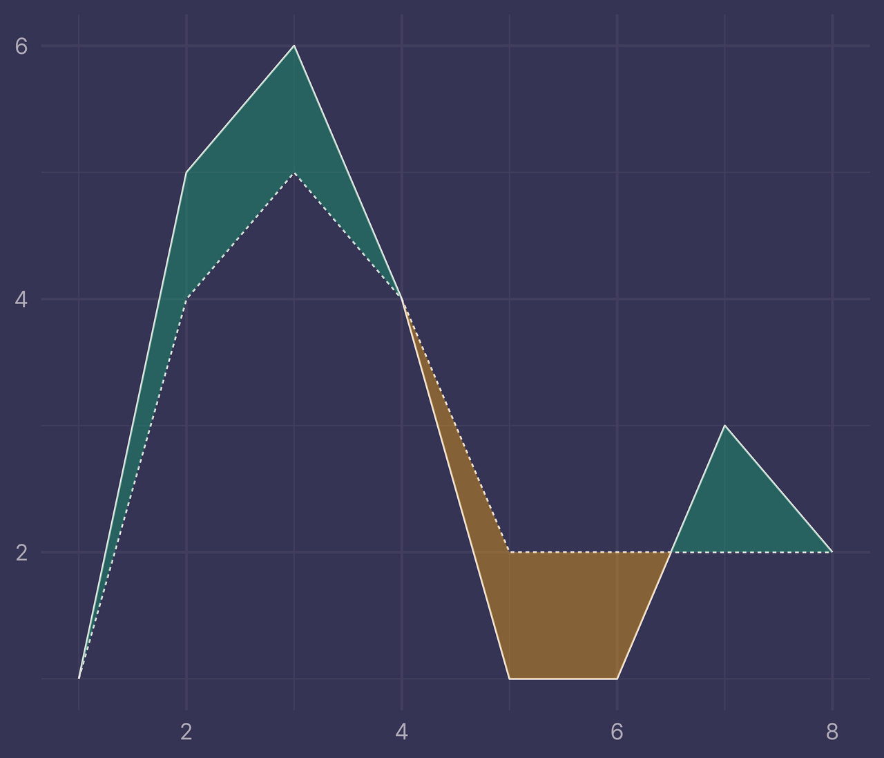
Voila!
Introducing ribbonize()
If you’d like to apply this to your own situation, I’ve written a function that reproduces all the same steps in this post.
I’ve called the function ribbonize(). Feel free to use it however you’d like — for the British English spellers, you have my permission to rename it to ribbonise(). :)
ribbonize <- function(.data, .x, .y, .f) {
  # Calculate the ribbons required for geom_ribbon().
  # For more info, visit nsgrantham.com/fill-between-two-lines-ggplot2
  #
  # Usage:
  # df <- tibble(
  #   x = c(1:8, 1:8),
  #   y = c(1, 5, 6, 4, 1, 1, 3, 2, 1, 4, 5, 4, 2, 2, 2, 2),
  #   f = c(rep("a", 8), rep("b", 8))
  # )
  #
  # ribbons <- ribbonize(df, x, y, f)
  #
  # ggplot(df) +
  #   geom_line(aes(x, y, linetype = f)) +
  #   geom_ribbon(data = ribbons, aes(x, ymin = ymin, ymax = ymax, fill = fill))

  # Check there are only 2 level in .f
  levels <- .data %>%
    pull({{ .f }}) %>%
    unique()

  stopifnot(length(levels) == 2)

  # Check that there is exactly 1 observation per level in .f at every .x
  level_counts_by_x <- .data %>%
    filter(!is.na({{ .y }})) %>%
    group_by({{ .x }}) %>%
    count() %>%
    pull(n)

  stopifnot(all(level_counts_by_x == 2))

  bounds <- .data %>%
    mutate({{ .f }} := recode({{ .f }}, a = levels[1], b = levels[2])) %>%
    pivot_wider(names_from = {{ .f }}, values_from = {{ .y }}) %>%
    mutate(
      ymax = pmax(a, b),
      ymin = pmin(a, b),
      fill = a >= b
    )

  intervals <- bounds %>%
    filter(ymax > ymin) %>%
    select(-a, -b)

  intersections <- bounds %>%
    mutate(lag_fill = lag(fill), lead_fill = lead(fill)) %>%
    filter(ymax == ymin) %>%
    select(-a, -b, -fill) %>%
    pivot_longer(lag_fill:lead_fill, names_to = NULL, values_to = "fill") %>%
    filter(!is.na(fill)) %>%
    distinct()

  other_intersections <- bounds %>%
    transmute(
      x1 = {{ .x }},       y1 = a,
      x2 = lead({{ .x }}), y2 = lead(a),
      x3 = {{ .x }},       y3 = b,
      x4 = lead({{ .x }}), y4 = lead(b)
    ) %>%
    filter(((y1 > y3) & (y2 < y4)) | ((y1 < y3) & (y2 > y4))) %>%
    mutate(
      d = (x1 - x2) * (y3 - y4) - (y1 - y2) * (x3 - x4),
      u = x1 * y2 - y1 * x2,
      v = x3 * y4 - y3 * x4,
      x = (u * (x3 - x4) - v * (x1 - x2)) / d,
      y = (u * (y3 - y4) - v * (y1 - y2)) / d
    ) %>%
    select(x, ymax = y, ymin = y)

  bind_rows(
    intervals,
    intersections,
    mutate(other_intersections, fill = TRUE),
    mutate(other_intersections, fill = FALSE)
  ) %>%
    arrange({{ .x }})
}
ribbons <- ribbonize(df, x, y, f)

ggplot(df) +
  geom_line(aes(x, y, linetype = f)) +
  geom_ribbon(data = ribbons, aes(x, ymin = ymin, ymax = ymax, fill = fill), alpha = 0.4) +
  guides(linetype = "none", fill = "none") +
  labs(x = NULL, y = NULL)

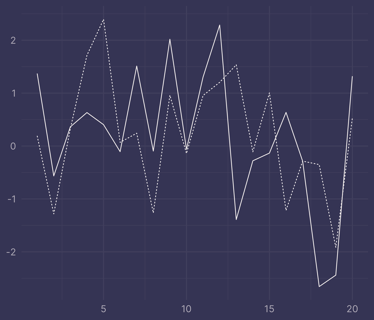
And for a sanity check, let’s try it out on a randomly generated dataset.
set.seed(42)  # for reproducibility

df <- tibble(
  x = c(1:20, 1:20),
  y = c(rnorm(20), rnorm(20, mean = 0.5)),
  f = c(rep("a", 20), rep("b", 20))
)

ggplot(df, aes(x, y, linetype = f)) +
  geom_line() +
  guides(linetype = "none") +
  labs(x = NULL, y = NULL)
ribbons <- ribbonize(df, x, y, f)

ggplot(df) +
  geom_line(aes(x, y, linetype = f)) +
  geom_ribbon(data = ribbons, aes(x, ymin = ymin, ymax = ymax, fill = fill), alpha = 0.4) +
  guides(linetype = "none", fill = "none") +
  labs(x = NULL, y = NULL)
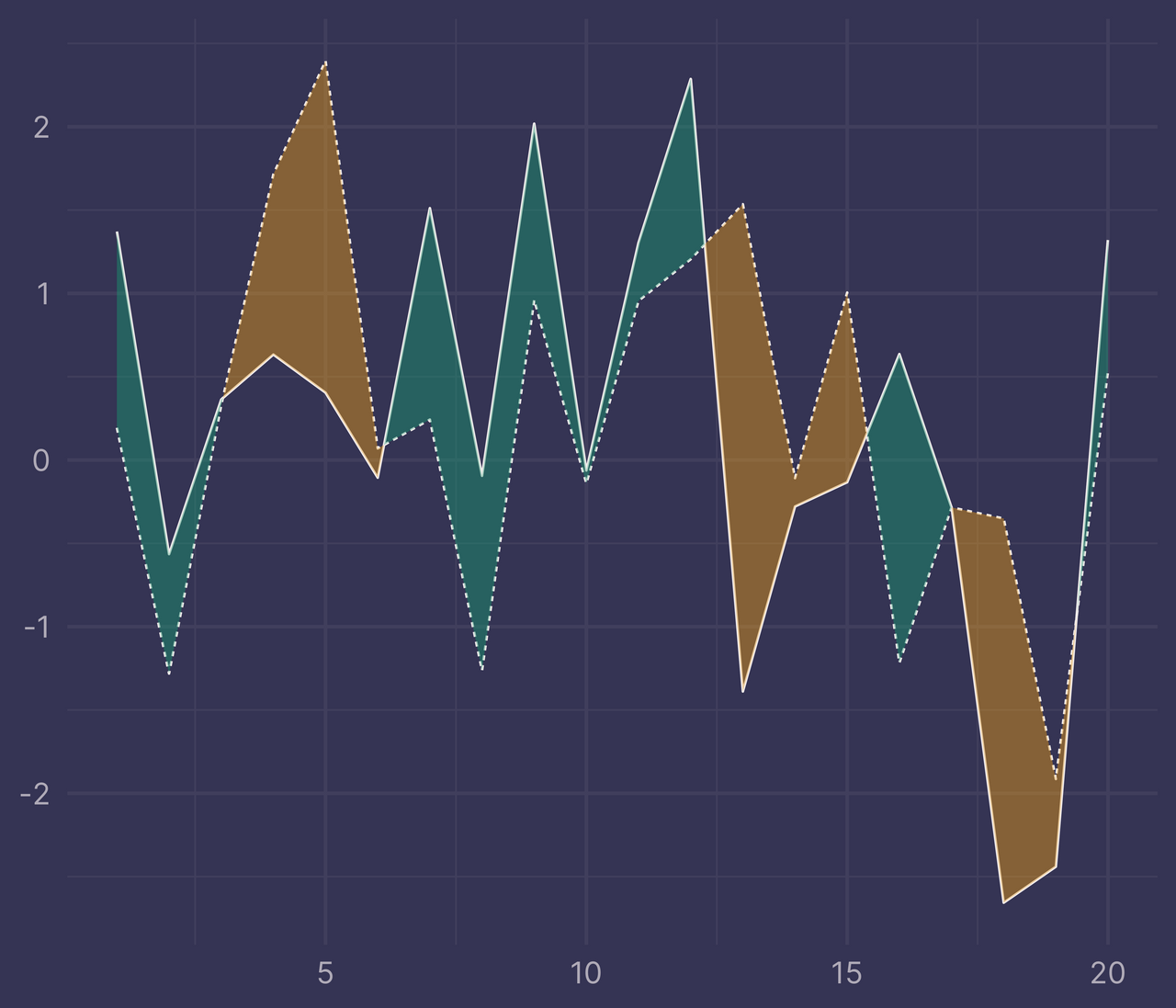
Perfecto!
When doesn’t this work?
ribbonize() has a couple requirements to work properly.
First, it only works for data with exactly two factor levels. Any more, or any less, and it will throw an error.
df <- tibble(
  x = c(1:6, 1:6, 1:6),
  y = c(1, 5, 6, 4, 1, 1, 1, 4, 5, 4, 2, 2, 5, 2, 4, 2, 1, 3),
  f = c(rep("a", 6), rep("b", 6), rep("c", 6))
)

ggplot(df) +
  geom_line(aes(x, y, linetype = f)) +
  guides(linetype = "none") +
  labs(x = NULL, y = NULL)
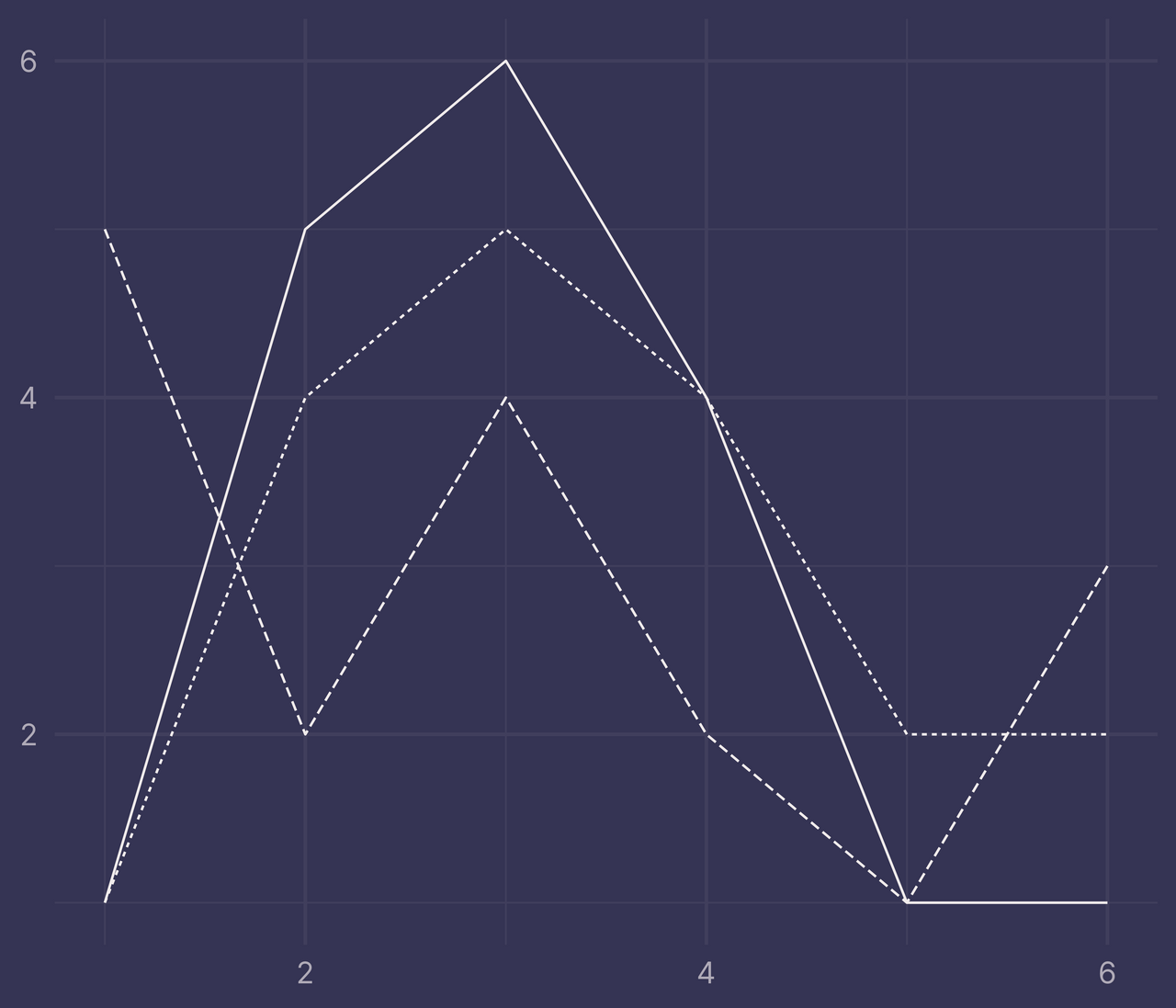
ribbons <- ribbonize(df, x, y, f)
## Error in ribbonize(df, x, y, f): length(levels) == 2 is not TRUE
Second, for every x in df there must be a corresponding value y for each level in f, otherwise ribbonize() will throw an error.
df <- tibble(
  x = c(1:6, 1:6),
  y = c(1, 5, 6, NA, 1, 1, 1, 4, 5, 4, NA, 2),
  f = c(rep("a", 6), rep("b", 6))
)

df
## # A tibble: 12 × 3
##        x     y f
##    <int> <dbl> <chr>
##  1     1     1 a
##  2     2     5 a
##  3     3     6 a
##  4     4    NA a
##  5     5     1 a
##  6     6     1 a
##  7     1     1 b
##  8     2     4 b
##  9     3     5 b
## 10     4     4 b
## 11     5    NA b
## 12     6     2 b
If we filter out the rows with NA and pass it to ggplot(), we can still plot it correctly (I added points with geom_point() so it’s easier to see where we’re missing data).
df %>%
  filter(!is.na(y)) %>%
  ggplot() +
  geom_line(aes(x, y, linetype = f)) +
  geom_point(aes(x, y)) +
  guides(linetype = "none") +
  labs(x = NULL, y = NULL)
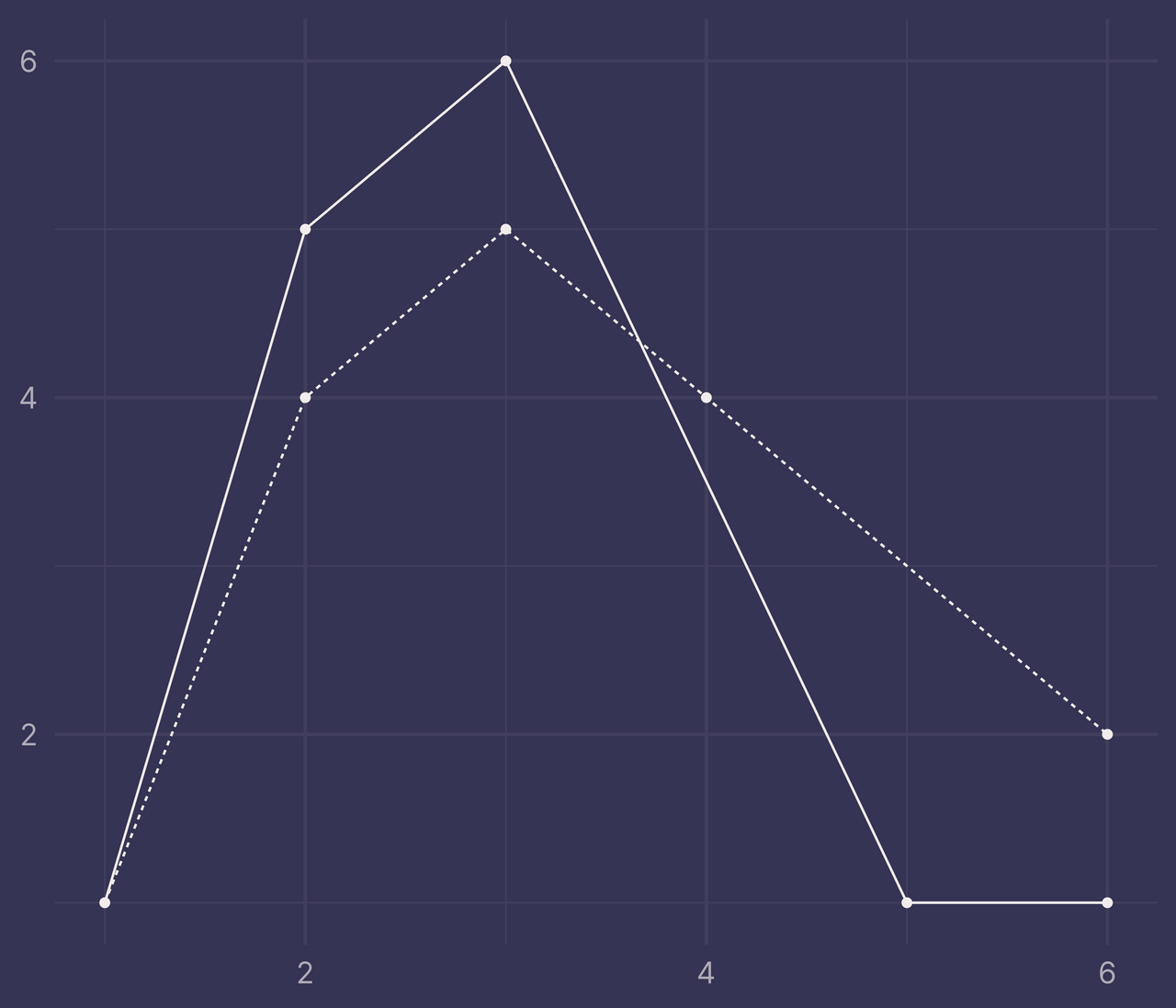
But if this same data is passed to ribbonize() it throws an error.
ribbons <- ribbonize(df, x, y, f)
## Error in ribbonize(df, x, y, f): all(level_counts_by_x == 2) is not TRUE
The function can be modified to accommodate data like this, but I’ll leave that work for a future blog post.
Wrapping Up
If you use ribbonize() in your own work and run into any issues, reach out to me on Twitter.
Happy ribbonizing! 🎀